DuckDB Internals: Query Planning and Columnar Storage Deep Dive

DuckDB has gone from a research project at CWI Amsterdam in 2019 to one of the most widely adopted databases of the past decade. It powers notebooks, ETL pipelines, dashboards, CI test runners, embedded analytics in SaaS products, and even an iPhone running TPC-H at scale factor 100 (source: MotherDuck). Companies like MotherDuck, Hex, Omni, Evidence, Fivetran, and Rill build products on top of it. At Greybeam, we use it for millions of BI queries.

Why In-Process Matters

DuckDB is an in-process analytical SQL database. Analytical means it's optimized for scanning millions of rows to filter, aggregate, and join — not single-record lookups. In-process means there's no server. You load it as a library, same as NumPy or Polars.

Most analytical databases are servers: Snowflake, Postgres, BigQuery, Redshift. They serialize every record into a wire protocol, transmit it over TCP, and deserialize on the client. In 2017, Mark Raasveldt and Hannes Mühleisen published "Don't Hold My Data Hostage," measuring that the client protocol itself — ODBC, JDBC — was often the slowest single step, sometimes dwarfing query computation time.

Two costs drive this. First, bandwidth: a gigabit Ethernet link caps at ~125 MB/s. Second, per-value overhead: ODBC/JDBC hand back results one row at a time, requiring a function call per field per row. On a 100-million-row result, that's hundreds of millions of calls.

DuckDB sidesteps both bottlenecks by living in the same process as the client. When a Python script runs con.sql("SELECT ... FROM my_df") against a pandas DataFrame, DuckDB uses a replacement scan. Instead of copying the DataFrame into an internal table, it reads from the DataFrame directly. In the best case, DuckDB reads the same underlying buffers the Python process already owns — zero-copy. If NumPy says "here's a buffer of 1 million int64 values," DuckDB can read that buffer directly because it understands the same physical layout. Arrow is the cleanest version: Arrow is already a columnar, typed memory format designed for sharing data between systems.

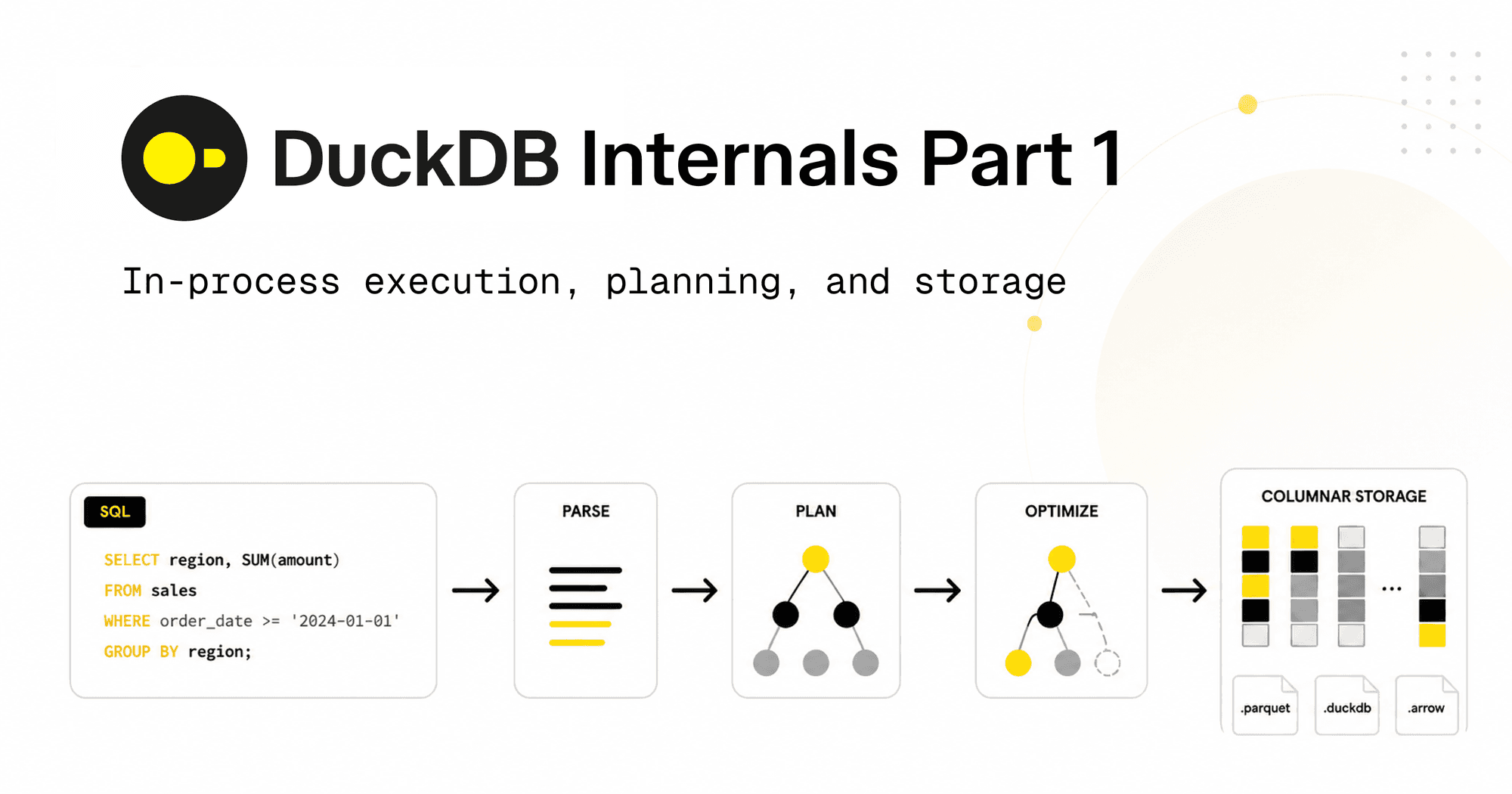
From SQL to Logical Plan

Once SQL reaches DuckDB, it goes through: parse, bind, plan, optimize.

Parsing

DuckDB uses a fork of the Postgres parser, so its dialect feels familiar. Parsing turns SELECT sum(l_quantity) FROM lineitem WHERE l_shipdate > '2024-01-01' into an abstract syntax tree (AST):

Select(
  expressions=[Sum(this=Column(this=Identifier(this=l_quantity, quoted=False)))],
  from_=From(this=Table(this=Identifier(this=lineitem, quoted=False))),
  where=Where(this=GT(this=Column(this=Identifier(this=l_shipdate, quoted=False)),
                       expression=Literal(this='2024-01-01', is_string=True))))

Binding

Binding resolves every name against the catalog. lineitem becomes a specific table with a known schema. l_quantity becomes a specific column with a known type. sum becomes a specific aggregate function. Type checking happens here: comparing l_shipdate to the string '2024-01-01' works because the binder coerces the literal to a date. The output is a bound tree where every node knows its type and what it refers to.

The Optimizer

DuckDB's optimizer consists of a sequence of small, focused transformations you can inspect and disable individually:

SELECT * FROM duckdb_optimizers();

This returns 33 optimizers, including filter_pushdown, join_order, statistics_propagation, and compressed_materialization. Running SET disabled_optimizers = 'filter_pullup, join_order' turns specific passes off.

Filter pushdown: Move WHERE predicates as close to the scan as possible to prune data early. DuckDB first pulls filters up to combine and reorganize them, then pushes them back down.

Subquery unnesting: Correlated subqueries are rewritten as joins using techniques from the "Unnesting Arbitrary Queries" paper, dramatically faster.

Dynamic join-filter pushdown: During a hash join, the build side must be fully read before the probe side starts. DuckDB computes the min and max of the join key values from the build side, then pushes those bounds back into the probe-side scan as a runtime filter. If the build side has values only between 100 and 200, the probe scan uses zonemaps to skip row groups outside that range. When the build side has fewer than 50 distinct join key values, the filter becomes an IN list instead of a min-max range, skipping even more rows.

Join order optimization: Join order determines intermediate result sizes. A query joining six tables has 30,240 possible orders. DuckDB uses a combination of heuristics and dynamic programming to find a good order.

Storage Layer: Columnar and Compressed

DuckDB stores data in columnar row groups. Each row group is a horizontal partition of the table, typically containing around 120,000 rows. Within a row group, each column is stored in a compressed, columnar format. This layout enables vectorized execution: operators process batches of values (vectors) instead of individual rows, which is CPU cache-friendly.

Zonemaps store the min and max values for each column in each row group. The query optimizer uses zonemaps to skip entire row groups during scans. For example, if you query WHERE l_shipdate > '2024-01-01', DuckDB can skip any row group whose max l_shipdate is before that date.

What's Next

This post covers the path from SQL to logical plan and the storage layer. Part 2 will cover query execution: vectorized processing, morsel-driven parallelism, and the runtime engine. Subscribe to the Greybeam blog for the full series.